
The only thing that stands in the way of perfection is the assumption we made that the friction loss in nonuniform flow at a given depth and discharge is the same as would be seen in the corresponding uniform flow at the same depth and discharge.
People do numerical integrations of Equation \ref to get approximate but reasonable water-surface profiles in real gradually varied flows. But what is also commonly done is just to use Equation \ref as a qualitative guide to the profile shape to be expected. We will do a little of that here, so that we can finally address the problem of what the water surface looks like as the river runs into the deep reservoir—and that is just one of the many important problems that can be attacked by this approach.
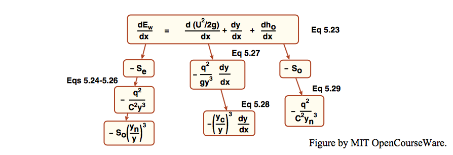
What you need to think about is the sign of \(dy/dx\) on the left side of Equation \ref, because if \(dy/dx\) is positive then the flow depth increases downstream, and if \(dy/dx\) is negative then the flow depth decreases downstream— and this is just the information we need in order to keep track of what the water surface does relative to the channel bottom.
The derivative \(dy/dx\) is positive (meaning that the depth increases downstream) if in Equation \ref both the numerator and the denominator are positive or if both the numerator and the denominator are negative. Conversely, \(dy/dx\) is negative, and the depth decreases downstream, if the numerator and the denominator have different sign.
Another thing we can do is think about the conditions under which
Suppose that our river flow is subcritical, as is usually the case for large rivers, meaning that the depth is greater than critical and the velocity is less than critical. We can express this by the condition \(y > y_\). So the denominator in the fraction in the right side of Equation \ref, which in the following I will call \(F\), is always less than one. With regard to the numerator, you know already that whatever the actual shape of the water-surface profile, the depth must ultimately increase when the reservoir is reached, so \(y > y_\) as well. Also, because we said that the approaching river is subcritical, you know that \(y_ > y_\). You can easily convince yourself that these three inequalities guarantee that the fraction \(F\) must be positive and less than one, so \(dy/dx\) is positive and less than \(S_>\), meaning that the depth gradually increases downstream.
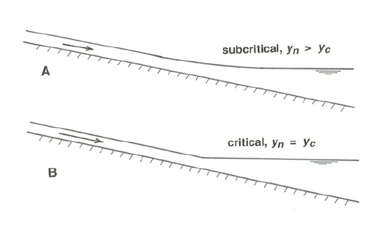
As \(y\) gets larger and larger in the process, both the numerator and the denominator of \(F\) go to one, meaning that \(dy/dx\) goes to \(S_>\), which if you think about it a little bit is the same as saying that the water surface itself becomes horizontal. So our conclusion is that the water-surface profile is as shown in Figure \(\PageIndex\)A: it is asymptotic to the uniform-flow profile upstream, and to the horizontal water surface of the reservoir downstream. This kind of curve is called a backwater curve, for reasons I suppose are obvious.
To carry this analysis just a little further, what is the effect of assuming that the river upstream is flowing at conditions closer to being critical? You can see by inspection of the fraction \(F\) that as \(y_ \rightarrow y_\), \(F\) itself stays closer and closer to one for \(y > y_\), meaning that the transition from the almost uniform flow upstream to the horizontal reservoir level downstream is sharper and sharper (that is, it takes place over a shorter and shorter distance), until, for critical flow upstream, the river meets the reservoir at a sharp angle (Figure \(\PageIndex\)B)!
For big rivers flowing well below the critical condition, the backwater effect is felt not just for kilometers but for tens of kilometers upstream, and the superelevation of the actual water surface above the hypothetical point of intersection between the uniform flow and the reservoir level can be many meters. You can imagine the importance of being able to predict the magnitude of this superelevation at all points upstream, when you are worrying about how many homes and farms and businesses you are going to be flooding when you build that dam.
I have just scratched the surface of the business of analyzing backwater effects. There are many qualitatively different kinds of backwater curves, depending upon whether the approaching flow is subcritical, critical, or supercritical, and upon whether
This page titled 5.7: Gradually Varied Flow is shared under a CC BY-NC-SA 4.0 license and was authored, remixed, and/or curated by John Southard (MIT OpenCourseware) via source content that was edited to the style and standards of the LibreTexts platform.